Multi-fidelity AI for wind engineering

Abstract

Computational fluid dynamics (CFD) represents an attractive tool for estimating wind pressures and wind loads on high-rise buildings. The CFD analyses can be conducted either by low-fidelity simulations (RANS) or by high-fidelity ones (LES). The low-fidelity model can efficiently estimate wind pressures over a large range of wind directions, but it generally lacks accuracy. On the other hand, the high-fidelity model generally exhibits satisfactory accuracy, yet, the high computational cost can limit the number of approaching wind angles that can be considered. In order to take advantage of the main benefits of these two CFD approaches, a multi-fidelity machine learning framework is investigated that aims to ensure the simulation accuracy while maintaining the computational efficiency. The study shows that the accurate prediction of distributions of mean and rms pressure over a high-rise building for the entire wind rose can be obtained by utilizing only 3 LES-related wind directions. The artificial neural network is shown to perform best among considered machine learning models. Moreover, hyperparameter optimization significantly improves the model predictions, increasing the value in the case of rms pressure by 60%. Dominant and ineffective features are determined that provide a route to solve a similar application more effectively.

Research question and experimental design

Wind-load assessment requires pressure estimates across many incident directions. Reynolds-averaged Navier–Stokes (RANS) simulations provide affordable directional coverage but do not resolve the unsteady fluctuations needed for reliable RMS pressure coefficients. Large-eddy simulation (LES) offers higher fidelity at substantially greater computational cost. The study asks how a small number of LES cases can be combined with a larger RANS dataset to predict both mean and RMS surface pressure across the wind rose.

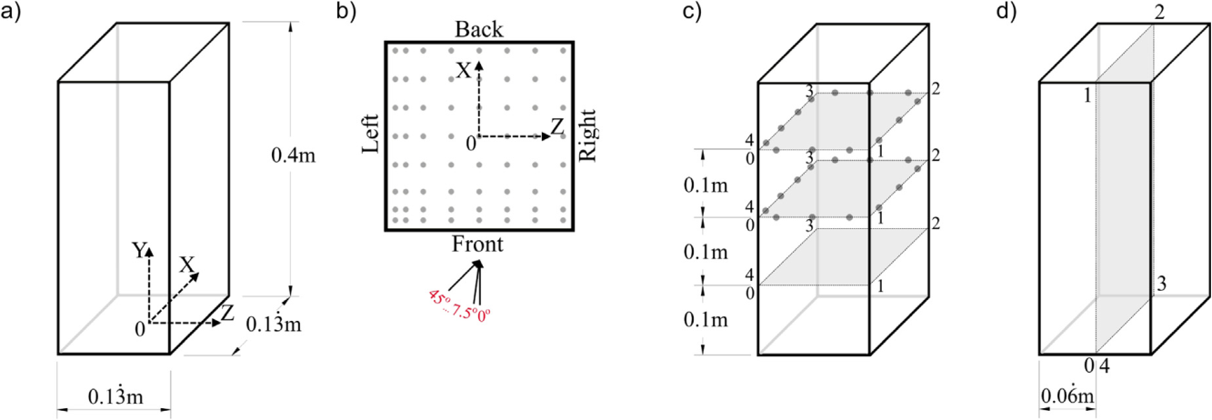
The benchmark is a square-section high-rise-building model with a 400 mm height and 133.33 mm width, representing a 120 m building at full scale. Seven directions—0°, 7.5°, 15°, 22.5°, 30°, 37.5° and 45°—cover the full wind rose by symmetry. Each direction contributes 7,153 surface points, up to nine input features and two targets: mean pressure coefficient C̄_p and RMS pressure coefficient C′_p.

High-rise-building geometry, coordinate system, wind-direction convention, and horizontal and vertical analysis planes — **Figure 1.** Building geometry and coordinate system; top view with the wind-direction convention; and the horizontal and vertical planes used for pressure analysis. Source: paper Figure 1.

Low-fidelity coverage: RANS simulations for all seven wind directions provide the input flow and pressure fields.
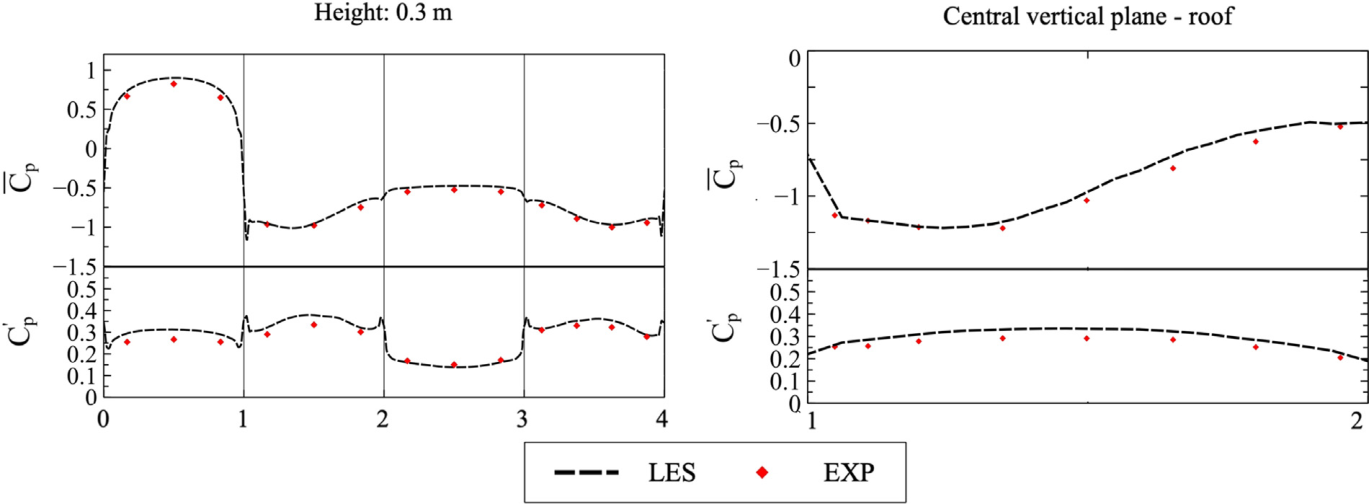
High-fidelity targets: LES supplies mean and RMS pressure coefficients and is validated against wind-tunnel measurements.
Adaptive training: The final universal model uses LES data at 0°, 22.5° and 45° to predict the intervening directions.

Methodology

Four regression families were evaluated: support vector machine, random forest, gradient boosting and an artificial neural network (ANN). Models were first trained on the two extreme directions, {0°, 45°}, and tested at 15°, the most difficult held-out case. The study then compared intermediate LES directions and selected {0°, 22.5°, 45°} as the final training set.

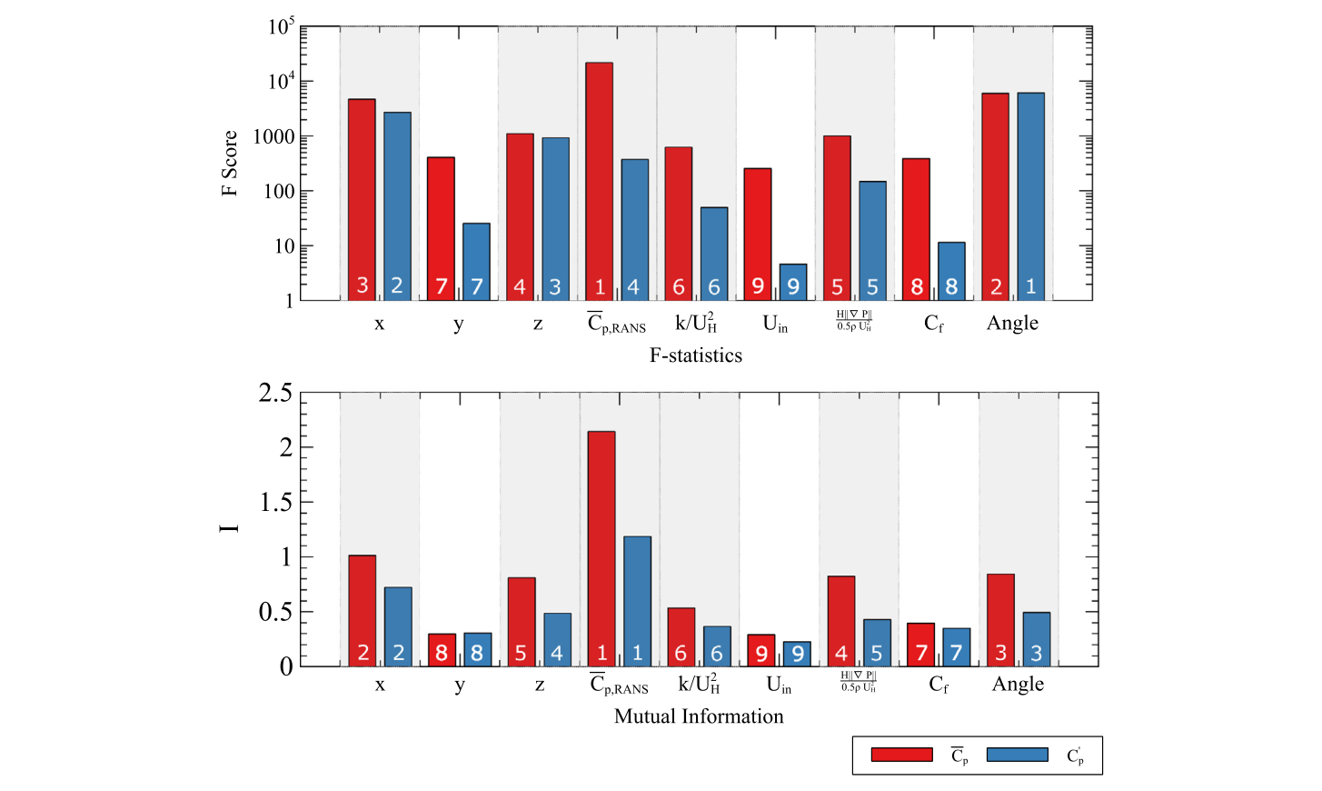
Input ablations begin with five flow features and add surface coordinates and wind direction. Hyperparameters were optimised separately for each model. A final feature-selection step used F-statistics and mutual information to identify six dominant inputs before testing the universal ANN at 15° and 30°.

LES and wind-tunnel mean and RMS pressure-coefficient profiles for the zero-degree wind direction — **Figure 6.** LES validation against wind-tunnel measurements at 0°. Mean and RMS pressure coefficients are compared around the building perimeter at 0.3 m height and along the middle roof line. Source: paper Figure 6.

F-statistics and mutual-information scores and ranks for nine wind-engineering input features — **Figure 12.** Feature selection using F-statistics and mutual information. The paper highlights the optimal six features in grey and reports each feature’s rank within the bars. Source: paper Figure 12.

Results

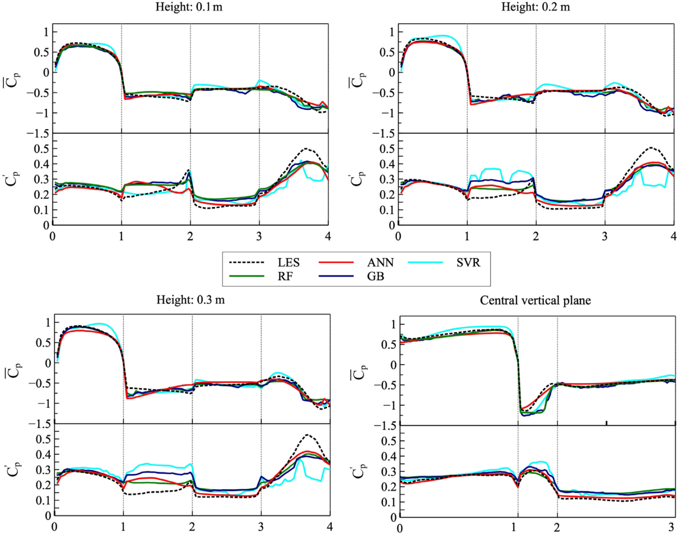
The ANN produced the strongest predictions in the difficult 15° test case. With all nine features, hyperparameter optimisation improved its RMS-pressure R² from 0.4358 to 0.5745 and reduced RMSE from 0.0803 to 0.0693. The complete model comparison reported in the paper is reproduced below.

LES and machine-learning model comparisons of mean and RMS surface-pressure coefficients at three heights and on the roof — **Figure 9.** LES and machine-learning predictions at 15° after training on {0°, 45°} with nine features. Profiles compare mean and RMS pressure coefficients at three heights around the building and along the central vertical plane. Source: paper Figure 9.

Model and feature-set comparison

**Table 2.** Test RMSE and R² for models trained on {0°, 45°} and tested at 15°, before and after hyperparameter optimisation.
Model	Feature set	Mean C̄_p				RMS C′_p
		Not optimised		Optimised		Not optimised		Optimised
		R²	RMSE	R²	RMSE	R²	RMSE	R²	RMSE
Support vector machine	5 flow features	0.9293	0.1464	0.9293	0.1464	−0.2264	0.1176	−0.2264	0.1176
	+ Angle	0.9352	0.1431	0.9352	0.1431	0.2589	0.0914	0.2589	0.0914
	+ Coordinates	0.9253	0.1512	0.9253	0.1512	0.1805	0.0961	0.1805	0.0961
	+ Coordinates + angle	0.9511	0.1224	0.9511	0.1224	0.4006	0.0822	0.4006	0.0822
Random forest	5 flow features	0.9295	0.1421	0.9381	0.1377	−0.2123	0.1169	−0.1887	0.1158
	+ Angle	0.9368	0.1399	0.9445	0.1304	0.2830	0.0908	0.2959	0.0891
	+ Coordinates	0.9301	0.1502	0.9416	0.1337	0.1846	0.0936	0.2097	0.0944
	+ Coordinates + angle	0.9532	0.1200	0.9581	0.1131	0.3840	0.0882	0.4223	0.0807
Gradient boosting	5 flow features	0.9321	0.1408	0.9501	0.1237	−0.1188	0.1123	−0.0855	0.1107
	+ Angle	0.9415	0.1313	0.9585	0.1127	0.3131	0.0880	0.3738	0.0841
	+ Coordinates	0.9403	0.1380	0.9512	0.1217	0.2908	0.1084	0.3573	0.0851
	+ Coordinates + angle	0.9524	0.1199	0.9613	0.1088	0.3936	0.0827	0.4403	0.0794
Artificial neural network	5 flow features	0.9469	0.1297	0.9515	0.1201	−0.1012	0.1078	0.0702	0.1024
	+ Angle	0.9588	0.1110	0.9668	0.1008	0.3994	0.0823	0.5046	0.0759
	+ Coordinates	0.9606	0.1098	0.9633	0.1051	0.3524	0.0978	0.4322	0.0800
	+ Coordinates + angle	0.9656	0.1002	0.9705	0.0951	0.4358	0.0803	0.5745	0.0693

The paper reports the same values before and after optimisation for support vector regression because its default parameters were optimal. Source: paper Table 2.

Selecting the third LES direction

Adding one intermediate high-fidelity case materially improved predictions over the two-direction baseline. Among the five candidates, 22.5° gave the highest average R² for both output variables.

**Table 4.** Test-average R² for the optimised ANN trained on different three-direction datasets with nine features.
Training directions	Mean C̄_p, average R²	RMS C′_p, average R²
0°, 7.5°, 45°	0.9566	0.6657
0°, 15°, 45°	0.9655	0.8296
0°, 22.5°, 45°	0.9832	0.8531
0°, 30°, 45°	0.9613	0.7856
0°, 37.5°, 45°	0.9577	0.6779

Average R² is calculated over the held-out directions for each training set. Bold identifies the best reported row. Source: paper Table 4.

Universal model and dominant features

The final ANN was trained on {0°, 22.5°, 45°}. The six-feature model retained or slightly improved the nine-feature result: at 30°, it achieved R² = 0.8861 and RMSE = 0.0352 for RMS pressure.

**Table 5.** Test RMSE and R² for the optimised ANN trained on {0°, 22.5°, 45°} and tested at 15° and 30°.
Feature set	15° test				30° test
Feature set	Mean R²	Mean RMSE	RMS R²	RMS RMSE	Mean R²	Mean RMSE	RMS R²	RMS RMSE
5 flow features	0.9653	0.1030	0.3672	0.0822	0.9672	0.0907	0.4769	0.0749
+ Angle	0.9717	0.0930	0.7985	0.0478	0.9759	0.0777	0.8611	0.0412
+ Coordinates	0.9708	0.0945	0.7849	0.0501	0.9796	0.0890	0.8308	0.0485
+ Coordinates + angle	0.9764	0.0871	0.8294	0.0438	0.9814	0.0701	0.8824	0.0355
6 dominant features	0.9768	0.0850	0.8256	0.0439	0.9812	0.0702	0.8861	0.0352

Mean columns refer to C̄_p; RMS columns refer to C′_p. Bold marks the entries emphasised here; all numeric values reproduce the paper. Source: paper Table 5.

Computational cost, scope and limitations

The fidelity gap is substantial: the paper reports approximately 5.65 × 10⁴ CPU hours for one LES wind direction, compared with about 20 CPU hours for one RANS simulation. Bootstrapping 100 ANN training samples required approximately 16.8 CPU hours on the stated eight-core workstation.

The benchmark is an isolated, centrosymmetric building without an urban neighbourhood. Changes in geometry or surroundings may require retraining, and the authors identify transfer learning as a route towards broader reuse. The ANN remains a black-box predictor, and the reported outputs are mean and RMS pressure coefficients rather than peak pressure.

Technology and data

RANS and LES computational-fluid-dynamics surface fields; wind-tunnel validation data; Python and scikit-learn models including support vector regression, random forest and gradient boosting; an artificial neural network; hyperparameter optimisation; F-statistics and mutual-information feature selection; and evaluation with R² and RMSE.

BibTeX

@article{Glumac2023MultifidelityWind,
  author  = {Glumac, Anina {\v{S}}arki{\'c} and Jadhav, Onkar and Despotovi{\'c}, Vladimir and Blocken, Bert and Bordas, Stephane P. A.},
  title   = {A Multi-Fidelity Wind Surface Pressure Assessment via Machine Learning: A High-Rise Building Case},
  journal = {Building and Environment},
  volume  = {234},
  pages   = {110135},
  year    = {2023},
  month   = apr,
  doi     = {10.1016/j.buildenv.2023.110135},
  url     = {https://doi.org/10.1016/j.buildenv.2023.110135}
}

Citation metadata from the official journal record.

Research outputs

Anina Šarkić Glumac, Onkar Jadhav, Vladimir Despotović, Bert Blocken and S. P. A. Bordas, “A multi-fidelity wind surface pressure assessment via machine learning: A high-rise building case,” Building and Environment, 234, 110135 (2023).

The research was also presented at ECCOMAS, WCCM-APCOM and 8EACWE.